HIP:Mashup
Jump to navigation
Jump to search
Getting to the final mashup
This is an easy step by step procedure for converting data collected by sonde into the YSI 650 MDS and transfered into a computer to the pictures as seen below.
The following is an example of data from sonde, which has been converted to a csv file using EcoWatch.
"Date","Time","Temp","SpCond","Cond","Resistivity","pH","ORP","Longitude","Latitude"
"M/D/Y","hh:mm:ss","C","uS/cm","uS/cm","Ohm.cm","","mV","DD.dddd","DD.dddd"
"05/25/09","11:20:54",23.13,614.0,592.0,1688.4,8.98,145,-84.899391,39.848564
"05/25/09","11:21:04",23.14,616.0,594.0,1682.3,8.97,24,-84.899391,39.848560
"05/25/09","11:21:14",23.16,618.0,596.0,1677.6,8.92,10,-84.899406,39.848568
"05/25/09","11:21:24",23.23,616.0,596.0,1679.0,9.13,-8,-84.899414,39.848614
"05/25/09","11:21:34",23.30,615.0,595.0,1682.0,9.71,-3,-84.899445,39.848648
"05/25/09","11:21:44",23.31,614.0,594.0,1682.8,10.10,7,-84.899544,39.848686
"05/25/09","11:21:54",23.29,614.0,594.0,1683.5,10.28,14,-84.899628,39.848701
"05/25/09","11:22:04",23.21,615.0,594.0,1684.6,10.37,20,-84.899734,39.848736
"05/25/09","11:22:14",23.14,617.0,595.0,1681.2,10.38,24,-84.899818,39.848812
"05/25/09","11:22:24",23.09,617.0,595.0,1680.9,10.41,28,-84.899948,39.848873
"05/25/09","11:22:34",23.01,620.0,596.0,1677.1,10.39,32,-84.900017,39.848980
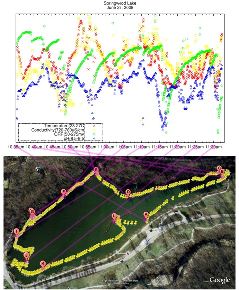
The final product from the cvs file is presented as the pictures below, which was produced from a combination of google earth, GNUplot and GNU Image Manipulation Program (GIMP).
- GNUplot which is used to get the graph is installed in all the ACLs and in stewie, and hence you don't have to install to use it.
- To make the graph, go to the directory where you have your data file (which will be a csv file if it was generated by EcoWatch).
- Into that directory, copy the following script and make adjustments for the name of your data file and the the ranges for your parameters.
- type "gnuplot" and return.
- To plot the data file type 'load "script name"' and enter.
- Here is the script:
#!/usr/local/bin/gnuplot]
reset
set terminal x11
#set output "aaa.png"
set datafile separator ","
set xdata time
set timefmt "%H:%M:%S"
set xrange ["11:20:50":"11:38:00"]
set format "%H:%Mam"
set title "Springwood Lake\nMay 25, 2009"
set multiplot
unset ytics
plot [][22:24]          "MIK2.csv" using 2:3\
                        notitle with p lt rgb "red" pt 2 #Temp
plot [][600:650]        "MIK2.csv" using 2:4\
                        notitle with p lt rgb "yellow" pt 4 #Cond
plot [][0:100]          "MIK2.csv" using 2:8\
                        notitle with p lt rgb "green" pt 6 #ORP
plot [][9.6:10.65]      "MIK2.csv" using 2:7\
                        notitle with p lt rgb "blue" pt 8 #pH
set key bottom left
set key box lt 5 lw 2
replot  "MIK2.csv" using 1:(1/0)\
         title "Temperature(22-24C)" with p lt rgb "red" pt 2,\
        "MIK2.csv" using 1:(1/0)\
         title "Conductivity(600-650uS/cm)" with p lt rgb "yellow" pt 4,\
        "MIK2.csv" using 1:(1/0)\
         title "ORP(0-100mv)" with p lt rgb "green" pt 6,\
        "MIK2.csv" using 1:(1/0)\
         title "pH(9.6-10.65)" with p lt rgb "blue" pt 8
unset multiplot

#EOF
- Next you want to get a satellite picture showing exactly where you took you data. To get this, you have to go to the directory where you have you data file from the YSI 650 MDS.
- Copy the following perl script into the same directory.
#!/usr/bin/perl
#Written by: Mikio Takizawa
#July 2008
#
#Modified in May 2009
#
#This script is for converting csv file, which is the data from
#springwood database, to kml file.
#
#
#Sample basic structure of kml file
#
#<?xml version="1.0" encoding="UTF-8"?>
#<kml xmlns="http://earth.google.com/kml/2.2">
#  <Placemark>
#    <name>Simple placemark</name>
#    <description>Attached to the ground. Intelligently places itself
#       at the height of the underlying terrain.</description>
#    <Point>
#      <coordinates>-122.0822035425683,37.42228990140251,0</coordinates>
#    </Point>
#  </Placemark>
#</kml>

use strict;

$ARGV[1] or die "Usage: $0 <infile> <outfile>\n";

my $infile = $ARGV[0];
my $outfile = $ARGV[1];
my $i;
my $j;
my $k;
my $l;
my $sdate;
- Run the scrip on you data file and send the out put to an output file.
- eg:
wir059151:untitled folder sanelemahlalela$ ls
MIK2.csv		sanele2.kml		ysi650_2_kml.pl		ysi650_2_plot.gplot
wir059151:untitled folder sanelemahlalela$ perl ysi650_2_kml.pl MIK2.csv sanele3.kml
Choose date from: "Date" "M/D/Y" "05/25/09"
Which one?: "05/25/09"
"05/25/09"
sanele3.kml is ready.
wir059151:untitled folder sanelemahlalela$
- Copy the kml file to your www directory in you home directory on quark.
- Copy that same file from your www directory onto your desktop.
- Now you can open google earth drag the file from your desktop and drop it on google earth.
- Sometimes you might have to zoom into the picture to see it clear (it will be indicated by a pin(s).
- There are a number of way which can be used to copy the picture from google earth to your desktop.
- One of them, which is the one I used is taking a snap shot of my desktop using the splat key + 4 on my apple computer.
- That picture is now ready to be integrated with the gnuplot we made using the GNUplot software.
- To Do the integration we use the GNU Image Manipulation Program mentioned above.
- Before doing that however, lets look into another way of getting our kml file into a satellite picture.
- We are going to use google maps instead of google earth.
- In this case you go to google maps. In the search bar, type "http://cs.earlham.edu/~stmahla07/sanele2.kml" enter ( substitute stmahla07 for earlham username(home directory on quark) and sanele2.kml for file name).
- Here you will get something similar to what google earth will give you. And again, you can copy the image onto your desktop in a number of ways including taking a snapshot of your desktop.
- Doing the real Mashup!
--to be continued.
