Difference between revisions of "HIP:Mashup"
Jump to navigation
Jump to search
| (38 intermediate revisions by 2 users not shown) | |||
| Line 1: | Line 1: | ||
| − | + | '''Getting to the final mashup'''<br> | |
| − | + | ''This is an easy step by step procedure for converting data collected by sonde from the YSI 650 MDS and transfering the data into a computer to | |
| − | + | ''get the pictures at the bottom of the page.''<br> | |
| + | ''The following is an example of data from sonde, which has been converted to a csv file using EcoWatch.''<br> | ||
| + | |||
| + | |||
<pre> | <pre> | ||
| − | + | "Date","Time","Temp","SpCond","Cond","Resistivity","pH","ORP","Longitude","Latitude" | |
| − | + | "M/D/Y","hh:mm:ss","C","uS/cm","uS/cm","Ohm.cm","","mV","DD.dddd","DD.dddd" | |
| − | + | "05/25/09","11:20:54",23.13,614.0,592.0,1688.4,8.98,145,-84.899391,39.848564 | |
| − | + | "05/25/09","11:21:04",23.14,616.0,594.0,1682.3,8.97,24,-84.899391,39.848560 | |
| + | "05/25/09","11:21:14",23.16,618.0,596.0,1677.6,8.92,10,-84.899406,39.848568 | ||
| + | "05/25/09","11:21:24",23.23,616.0,596.0,1679.0,9.13,-8,-84.899414,39.848614 | ||
| + | "05/25/09","11:21:34",23.30,615.0,595.0,1682.0,9.71,-3,-84.899445,39.848648 | ||
| + | "05/25/09","11:21:44",23.31,614.0,594.0,1682.8,10.10,7,-84.899544,39.848686 | ||
| + | "05/25/09","11:21:54",23.29,614.0,594.0,1683.5,10.28,14,-84.899628,39.848701 | ||
| + | "05/25/09","11:22:04",23.21,615.0,594.0,1684.6,10.37,20,-84.899734,39.848736 | ||
| + | "05/25/09","11:22:14",23.14,617.0,595.0,1681.2,10.38,24,-84.899818,39.848812 | ||
| + | "05/25/09","11:22:24",23.09,617.0,595.0,1680.9,10.41,28,-84.899948,39.848873 | ||
| + | "05/25/09","11:22:34",23.01,620.0,596.0,1677.1,10.39,32,-84.900017,39.848980 | ||
</pre> | </pre> | ||
| + | |||
| + | ''The final product from the cvs file is presented as the pictures below, which was produced from a combination of google earth, GNUplot and GNU Image Manipulation Program (GIMP).''<br> | ||
| + | |||
| + | [[Image:MashupExample.jpg]] | ||
| + | |||
| + | * GNUplot which is used to get the graph is installed in all the ACLs and in stewie, and hence you don't have to install to use it.<br> | ||
| + | * To make the graph, go to the directory where you have your data file (which will be a csv file if it was generated by EcoWatch).<br> | ||
| + | *Into that directory, copy the following script and make adjustments for the name of your data file and the the ranges for your parameters. | ||
| + | *type "gnuplot" and return.<br> | ||
| + | *set an output file where you want gnuplot to save your plot. save it as png or jpeg or something similar. | ||
| + | *To plot the data file type 'load "script name"' and enter.<br> | ||
| + | *Here is the script: | ||
| + | <pre> | ||
| + | #!/usr/local/bin/gnuplot] | ||
| + | reset | ||
| + | set terminal x11 | ||
| + | #set output "aaa.png" | ||
| + | set datafile separator "," | ||
| + | set xdata time | ||
| + | set timefmt "%H:%M:%S" | ||
| + | set xrange ["11:20:50":"11:38:00"] | ||
| + | set format "%H:%Mam" | ||
| + | set title "Springwood Lake\nMay 25, 2009" | ||
| + | set multiplot | ||
| + | unset ytics | ||
| + | plot [][22:24] "MIK2.csv" using 2:3\ | ||
| + | notitle with p lt rgb "red" pt 2 #Temp | ||
| + | plot [][600:650] "MIK2.csv" using 2:4\ | ||
| + | notitle with p lt rgb "yellow" pt 4 #Cond | ||
| + | plot [][0:100] "MIK2.csv" using 2:8\ | ||
| + | notitle with p lt rgb "green" pt 6 #ORP | ||
| + | plot [][9.6:10.65] "MIK2.csv" using 2:7\ | ||
| + | notitle with p lt rgb "blue" pt 8 #pH | ||
| + | set key bottom left | ||
| + | set key box lt 5 lw 2 | ||
| + | replot "MIK2.csv" using 1:(1/0)\ | ||
| + | title "Temperature(22-24C)" with p lt rgb "red" pt 2,\ | ||
| + | "MIK2.csv" using 1:(1/0)\ | ||
| + | title "Conductivity(600-650uS/cm)" with p lt rgb "yellow" pt 4,\ | ||
| + | "MIK2.csv" using 1:(1/0)\ | ||
| + | title "ORP(0-100mv)" with p lt rgb "green" pt 6,\ | ||
| + | "MIK2.csv" using 1:(1/0)\ | ||
| + | title "pH(9.6-10.65)" with p lt rgb "blue" pt 8 | ||
| + | unset multiplot | ||
| + | |||
| + | #EOF | ||
| + | </pre> | ||
| + | *Next you want to get a satellite picture showing exactly where you took you data. To get this, you have to go to the directory where you have you data file from the YSI 650 MDS. | ||
| + | *Copy the following perl script into the same directory. | ||
| + | <pre> | ||
| + | #!/usr/bin/perl | ||
| + | #Written by: Mikio Takizawa | ||
| + | #July 2008 | ||
| + | # | ||
| + | #Modified in May 2009 | ||
| + | # | ||
| + | #This script is for converting csv file, which is the data from | ||
| + | #springwood database, to kml file. | ||
| + | # | ||
| + | # | ||
| + | #Sample basic structure of kml file | ||
| + | # | ||
| + | #<?xml version="1.0" encoding="UTF-8"?> | ||
| + | #<kml xmlns="http://earth.google.com/kml/2.2"> | ||
| + | # <Placemark> | ||
| + | # <name>Simple placemark</name> | ||
| + | # <description>Attached to the ground. Intelligently places itself | ||
| + | # at the height of the underlying terrain.</description> | ||
| + | # <Point> | ||
| + | # <coordinates>-122.0822035425683,37.42228990140251,0</coordinates> | ||
| + | # </Point> | ||
| + | # </Placemark> | ||
| + | #</kml> | ||
| + | |||
| + | use strict; | ||
| + | |||
| + | $ARGV[1] or die "Usage: $0 <infile> <outfile>\n"; | ||
| + | |||
| + | my $infile = $ARGV[0]; | ||
| + | my $outfile = $ARGV[1]; | ||
| + | my $i; | ||
| + | my $j; | ||
| + | my $k; | ||
| + | my $l; | ||
| + | my $sdate; | ||
| + | </pre> | ||
| + | *Run the scrip on you data file and send the out put to an output file. | ||
| + | *eg: | ||
| + | <pre> | ||
| + | wir059151:untitled folder sanelemahlalela$ ls | ||
| + | MIK2.csv sanele2.kml ysi650_2_kml.pl ysi650_2_plot.gplot | ||
| + | wir059151:untitled folder sanelemahlalela$ perl ysi650_2_kml.pl MIK2.csv sanele3.kml | ||
| + | Choose date from: "Date" "M/D/Y" "05/25/09" | ||
| + | Which one?: "05/25/09" | ||
| + | "05/25/09" | ||
| + | sanele3.kml is ready. | ||
| + | wir059151:untitled folder sanelemahlalela$ | ||
| + | </pre> | ||
| + | *Copy the kml file to your www directory in your home directory on quark. | ||
| + | *Copy that same file from your www directory onto your desktop. | ||
| + | *Now you can open google earth, drag the file from your desktop and drop it on google earth. | ||
| + | *Sometimes you might have to zoom into the picture to see it clear (it will be indicated by a pin(s). | ||
| + | *There are a number of ways that can be used to copy the picture from google earth to your desktop. | ||
| + | * One of them, which is the one I used is taking a snap shot of the desktop using the shift + command + 4 on an apple computer. | ||
| + | *That picture is now ready to be integrated with the gnuplot we made using the GNUplot software. | ||
| + | *To Do the integration we use the GNU Image Manipulation Program mentioned above. | ||
| + | *Before doing that however, lets look into another way of getting our kml file into a satellite picture. | ||
| + | *We are going to use google maps instead of google earth. | ||
| + | *In this case you go to google maps. In the search bar, type "http://cs.earlham.edu/~stmahla07/sanele2.kml" enter ( substitute stmahla07 for earlham username(home directory on quark) and sanele2.kml for file name). <br> | ||
| + | *Here you will get something similar to what google earth will give you. And again, you can copy the image onto your desktop in a number of ways including taking a snapshot of your desktop or just saving the whole image. | ||
| + | **Doing the real Mashup! | ||
| + | *To put the two images together, you'll use GNU Image Manipulation Program (GIMP), which you can download from online. | ||
| + | *Open GIMP, open a new file and set the width and height. You want these to be big so that you can have an easier time drawing your lines and doing your mashup. | ||
| + | *open file. | ||
| + | *Open your picture from where you stored it (desktop). You want to open this as a layer and upload one to Gimp. | ||
| + | *Do the same for the other picture, open it as a layer on top of the first one ( see reference pics below). | ||
| + | *After every action, if the conversation box pops up with the option of scaling, select scale to save. | ||
| + | *On the menu bar on your GIMP, go to window -> dockable dialogs -> layers. A small box will pop up which have both of your layers and a blank. | ||
| + | *Push it to the side, you will need it soon. | ||
| + | *Go to the GIMP toolbox and select the scaling tool. | ||
| + | *Then select the top picture on your mashup and resize it from the sides, to half the size of you space. | ||
| + | *After resizing it, you can hold the picture from the center and pull it either down or up. | ||
| + | *On the small box with your layers (the one I said we will need soon), select your other picture, and do the same resizing and move it either up or down, as you would like it to be. | ||
| + | *To draw the lines, matching the time on the gnuplot and the points on the google picture that corresponds with that time, you will use the paint brush. Select the color you want. | ||
| + | *Now you can start drawing the lines. | ||
| + | *At this moment, you will realize that when you draw from one picture you can't move over to the other one. To do this, go to your small box, select the other picture, and then you can make you line through it. | ||
| + | *You will also realize that the lines you are drawing at the moment are not as straight as you would like them to be. To get straight lines, make a dot on one point, while holding shift key down, make a line to the other part of the picture where you want your line to go. Don't release your shift yet, right click on your track pad and then let go of the shift. | ||
| + | *To avoid having to go to the different layers, you can merge your pictures into one, which you will eventually want to do anyways to create one picture. Go to Layers -> merge down and draw your lines. | ||
| + | *Congratulations, you are done. | ||
| + | *Copy and save your mashup, and go make your poster. | ||
| + | Have a great day:) | ||
| + | |||
| + | See some reference pictures below. | ||
| + | <br> | ||
| + | [[Image:p3.png]] | ||
| + | <br> | ||
| + | <br> | ||
| + | [[Image:p4.png]] | ||
| + | <br> | ||
| + | <br> | ||
| + | [[Image:p5.png]] | ||
| + | <br> | ||
| + | <br> | ||
| + | [[Image:p6.png]] | ||
| + | <br> | ||
| + | <br> | ||
| + | [[Image:p7.png]] | ||
| + | <br> | ||
| + | <br> | ||
| + | [[Image:p8.png]] | ||
| + | <br> | ||
| + | <br> | ||
| + | [[Image:p9.png]] | ||
| + | <br> | ||
| + | <br> | ||
| + | [[Image:p10.png]] | ||
| + | <br> | ||
| + | |||
| + | --to be continued | ||
Latest revision as of 14:43, 6 September 2009
Getting to the final mashup
This is an easy step by step procedure for converting data collected by sonde from the YSI 650 MDS and transfering the data into a computer to
get the pictures at the bottom of the page.
The following is an example of data from sonde, which has been converted to a csv file using EcoWatch.
"Date","Time","Temp","SpCond","Cond","Resistivity","pH","ORP","Longitude","Latitude"
"M/D/Y","hh:mm:ss","C","uS/cm","uS/cm","Ohm.cm","","mV","DD.dddd","DD.dddd"
"05/25/09","11:20:54",23.13,614.0,592.0,1688.4,8.98,145,-84.899391,39.848564
"05/25/09","11:21:04",23.14,616.0,594.0,1682.3,8.97,24,-84.899391,39.848560
"05/25/09","11:21:14",23.16,618.0,596.0,1677.6,8.92,10,-84.899406,39.848568
"05/25/09","11:21:24",23.23,616.0,596.0,1679.0,9.13,-8,-84.899414,39.848614
"05/25/09","11:21:34",23.30,615.0,595.0,1682.0,9.71,-3,-84.899445,39.848648
"05/25/09","11:21:44",23.31,614.0,594.0,1682.8,10.10,7,-84.899544,39.848686
"05/25/09","11:21:54",23.29,614.0,594.0,1683.5,10.28,14,-84.899628,39.848701
"05/25/09","11:22:04",23.21,615.0,594.0,1684.6,10.37,20,-84.899734,39.848736
"05/25/09","11:22:14",23.14,617.0,595.0,1681.2,10.38,24,-84.899818,39.848812
"05/25/09","11:22:24",23.09,617.0,595.0,1680.9,10.41,28,-84.899948,39.848873
"05/25/09","11:22:34",23.01,620.0,596.0,1677.1,10.39,32,-84.900017,39.848980
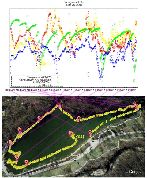
The final product from the cvs file is presented as the pictures below, which was produced from a combination of google earth, GNUplot and GNU Image Manipulation Program (GIMP).
- GNUplot which is used to get the graph is installed in all the ACLs and in stewie, and hence you don't have to install to use it.
- To make the graph, go to the directory where you have your data file (which will be a csv file if it was generated by EcoWatch).
- Into that directory, copy the following script and make adjustments for the name of your data file and the the ranges for your parameters.
- type "gnuplot" and return.
- set an output file where you want gnuplot to save your plot. save it as png or jpeg or something similar.
- To plot the data file type 'load "script name"' and enter.
- Here is the script:
#!/usr/local/bin/gnuplot]
reset
set terminal x11
#set output "aaa.png"
set datafile separator ","
set xdata time
set timefmt "%H:%M:%S"
set xrange ["11:20:50":"11:38:00"]
set format "%H:%Mam"
set title "Springwood Lake\nMay 25, 2009"
set multiplot
unset ytics
plot [][22:24]          "MIK2.csv" using 2:3\
                        notitle with p lt rgb "red" pt 2 #Temp
plot [][600:650]        "MIK2.csv" using 2:4\
                        notitle with p lt rgb "yellow" pt 4 #Cond
plot [][0:100]          "MIK2.csv" using 2:8\
                        notitle with p lt rgb "green" pt 6 #ORP
plot [][9.6:10.65]      "MIK2.csv" using 2:7\
                        notitle with p lt rgb "blue" pt 8 #pH
set key bottom left
set key box lt 5 lw 2
replot  "MIK2.csv" using 1:(1/0)\
         title "Temperature(22-24C)" with p lt rgb "red" pt 2,\
        "MIK2.csv" using 1:(1/0)\
         title "Conductivity(600-650uS/cm)" with p lt rgb "yellow" pt 4,\
        "MIK2.csv" using 1:(1/0)\
         title "ORP(0-100mv)" with p lt rgb "green" pt 6,\
        "MIK2.csv" using 1:(1/0)\
         title "pH(9.6-10.65)" with p lt rgb "blue" pt 8
unset multiplot

#EOF
- Next you want to get a satellite picture showing exactly where you took you data. To get this, you have to go to the directory where you have you data file from the YSI 650 MDS.
- Copy the following perl script into the same directory.
#!/usr/bin/perl
#Written by: Mikio Takizawa
#July 2008
#
#Modified in May 2009
#
#This script is for converting csv file, which is the data from
#springwood database, to kml file.
#
#
#Sample basic structure of kml file
#
#<?xml version="1.0" encoding="UTF-8"?>
#<kml xmlns="http://earth.google.com/kml/2.2">
#  <Placemark>
#    <name>Simple placemark</name>
#    <description>Attached to the ground. Intelligently places itself
#       at the height of the underlying terrain.</description>
#    <Point>
#      <coordinates>-122.0822035425683,37.42228990140251,0</coordinates>
#    </Point>
#  </Placemark>
#</kml>

use strict;

$ARGV[1] or die "Usage: $0 <infile> <outfile>\n";

my $infile = $ARGV[0];
my $outfile = $ARGV[1];
my $i;
my $j;
my $k;
my $l;
my $sdate;
- Run the scrip on you data file and send the out put to an output file.
- eg:
wir059151:untitled folder sanelemahlalela$ ls
MIK2.csv		sanele2.kml		ysi650_2_kml.pl		ysi650_2_plot.gplot
wir059151:untitled folder sanelemahlalela$ perl ysi650_2_kml.pl MIK2.csv sanele3.kml
Choose date from: "Date" "M/D/Y" "05/25/09"
Which one?: "05/25/09"
"05/25/09"
sanele3.kml is ready.
wir059151:untitled folder sanelemahlalela$
- Copy the kml file to your www directory in your home directory on quark.
- Copy that same file from your www directory onto your desktop.
- Now you can open google earth, drag the file from your desktop and drop it on google earth.
- Sometimes you might have to zoom into the picture to see it clear (it will be indicated by a pin(s).
- There are a number of ways that can be used to copy the picture from google earth to your desktop.
- One of them, which is the one I used is taking a snap shot of the desktop using the shift + command + 4 on an apple computer.
- That picture is now ready to be integrated with the gnuplot we made using the GNUplot software.
- To Do the integration we use the GNU Image Manipulation Program mentioned above.
- Before doing that however, lets look into another way of getting our kml file into a satellite picture.
- We are going to use google maps instead of google earth.
- In this case you go to google maps. In the search bar, type "http://cs.earlham.edu/~stmahla07/sanele2.kml" enter ( substitute stmahla07 for earlham username(home directory on quark) and sanele2.kml for file name).
- Here you will get something similar to what google earth will give you. And again, you can copy the image onto your desktop in a number of ways including taking a snapshot of your desktop or just saving the whole image.
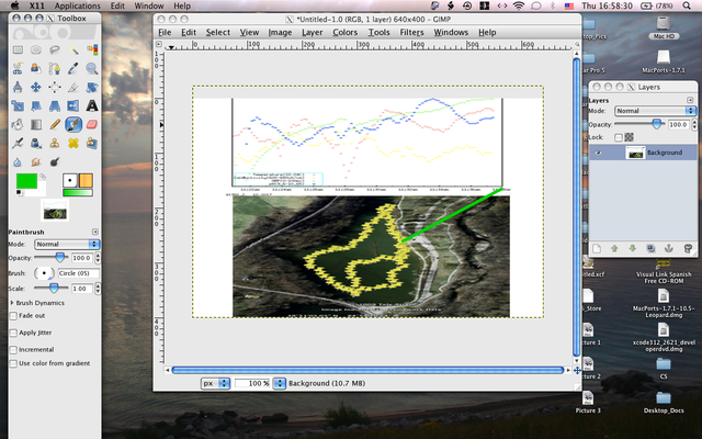
- Doing the real Mashup!
- To put the two images together, you'll use GNU Image Manipulation Program (GIMP), which you can download from online.
- Open GIMP, open a new file and set the width and height. You want these to be big so that you can have an easier time drawing your lines and doing your mashup.
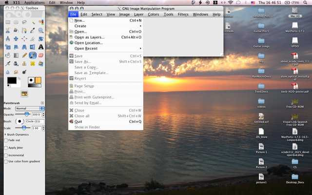
- open file.
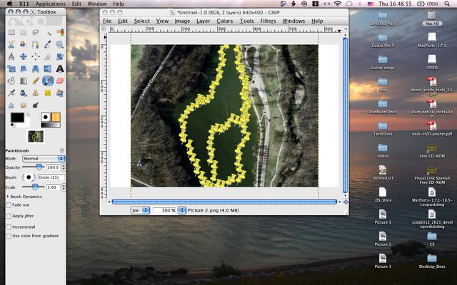
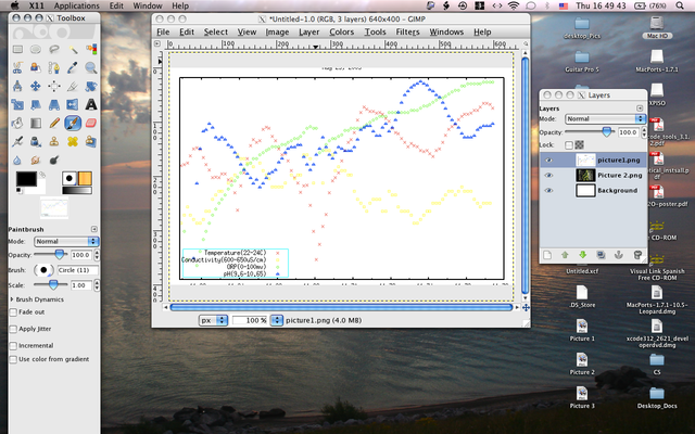
- Open your picture from where you stored it (desktop). You want to open this as a layer and upload one to Gimp.
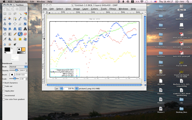
- Do the same for the other picture, open it as a layer on top of the first one ( see reference pics below).
- After every action, if the conversation box pops up with the option of scaling, select scale to save.
- On the menu bar on your GIMP, go to window -> dockable dialogs -> layers. A small box will pop up which have both of your layers and a blank.
- Push it to the side, you will need it soon.
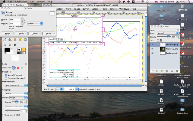
- Go to the GIMP toolbox and select the scaling tool.
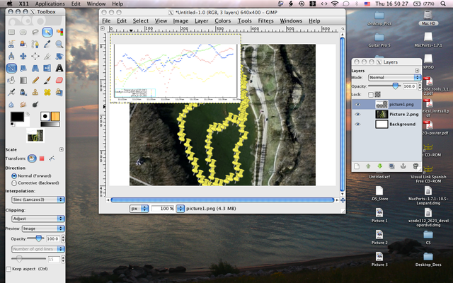
- Then select the top picture on your mashup and resize it from the sides, to half the size of you space.
- After resizing it, you can hold the picture from the center and pull it either down or up.
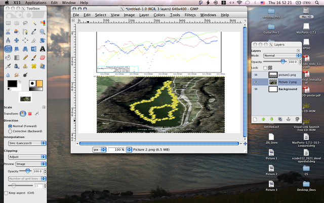
- On the small box with your layers (the one I said we will need soon), select your other picture, and do the same resizing and move it either up or down, as you would like it to be.
- To draw the lines, matching the time on the gnuplot and the points on the google picture that corresponds with that time, you will use the paint brush. Select the color you want.
- Now you can start drawing the lines.
- At this moment, you will realize that when you draw from one picture you can't move over to the other one. To do this, go to your small box, select the other picture, and then you can make you line through it.
- You will also realize that the lines you are drawing at the moment are not as straight as you would like them to be. To get straight lines, make a dot on one point, while holding shift key down, make a line to the other part of the picture where you want your line to go. Don't release your shift yet, right click on your track pad and then let go of the shift.
- To avoid having to go to the different layers, you can merge your pictures into one, which you will eventually want to do anyways to create one picture. Go to Layers -> merge down and draw your lines.
- Congratulations, you are done.
- Copy and save your mashup, and go make your poster.
Have a great day:)
See some reference pictures below.
--to be continued
